3 Working with graphics in GeoDa
3.1 Introduction
Today we are going to get acquaintanced with creating graphics for various statistic datasets in GeoDa. This GIS has prepared datasets and today we’ll use one of them. We’re going to work with Boston Housing 1970s, which contains housing and neighborhood data for the city of Boston based on research from the 1970s-90s. This dataset is a point shapefile with 506 observations and 23 variables. To open this data you have to choose File>New and to choose Boston Home Sales from Sample Data. After that you’ll be able to see the spatial distribution of the parameter. In the bottom left you’ll see the information about the number of observations.
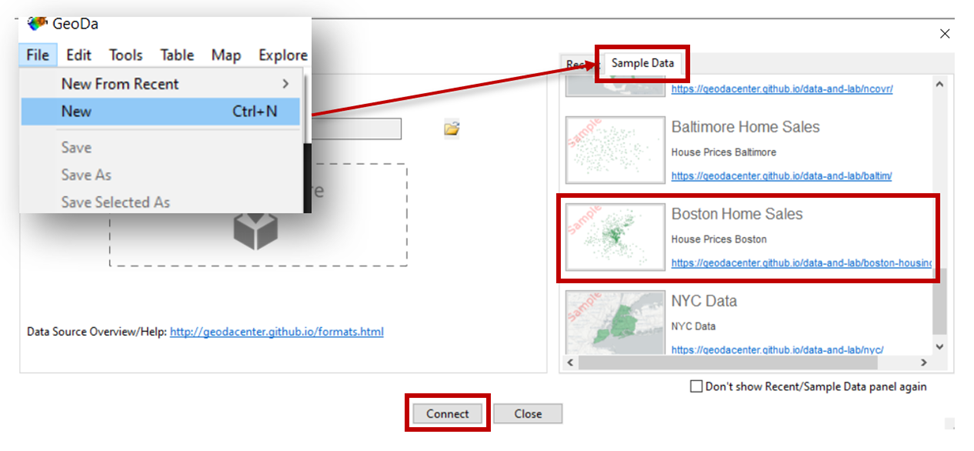
Figure 2.1: Opening the dataset
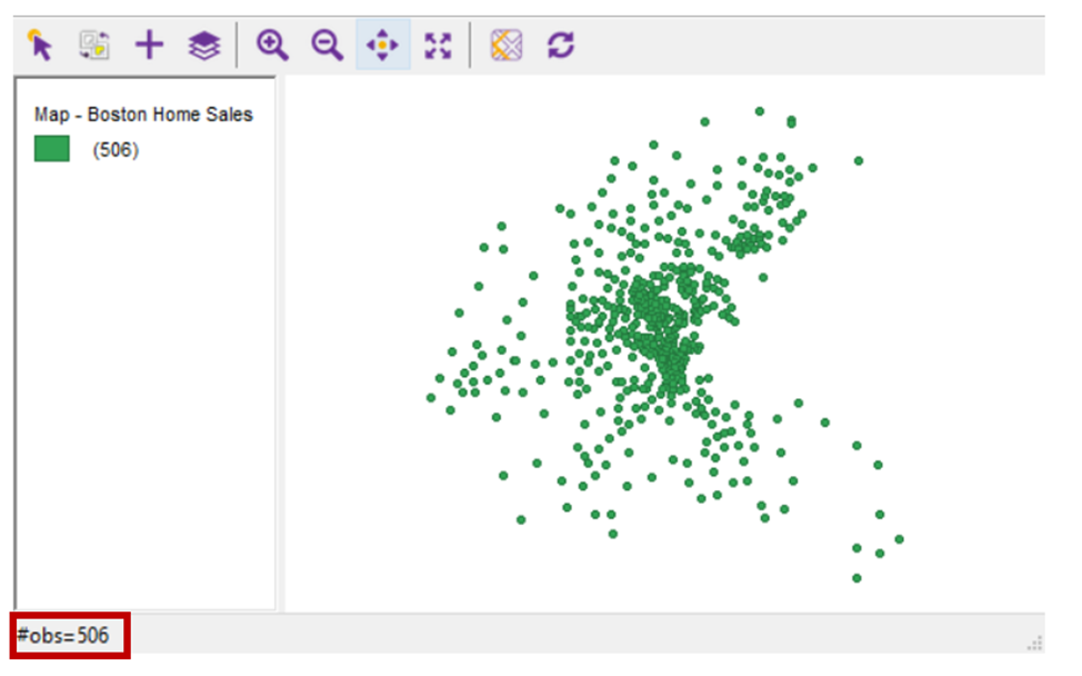
Figure 2.2: Boston Housing 1970s
3.2 Specific of data storage in GIS
To understand what observations and variables stand for we have to find out some facts about the ways of storing data in GIS. In GIS each object in a dataset consists of 2 parts: geometric (you see it) and semantic (responsible for the property of the object and represented as a row in a table). So, the semantic part is a table, where each line is an object of a dataset and each column contains the characteristic of the object. It means that the number of observations is a number of objects (rows) and the number of variables stands for the number of object characteristics (columns).
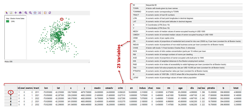
Figure 2.3: Storing data in GIS
3.3 Graphic types in GeoDa
There’re 8 types of graphics in GeoDA: Histogram, Box Plot, Scatter Plot, Scatter Plot, Matrix, Bubble Chart, 3D Scatter Plot, Conditional Plot
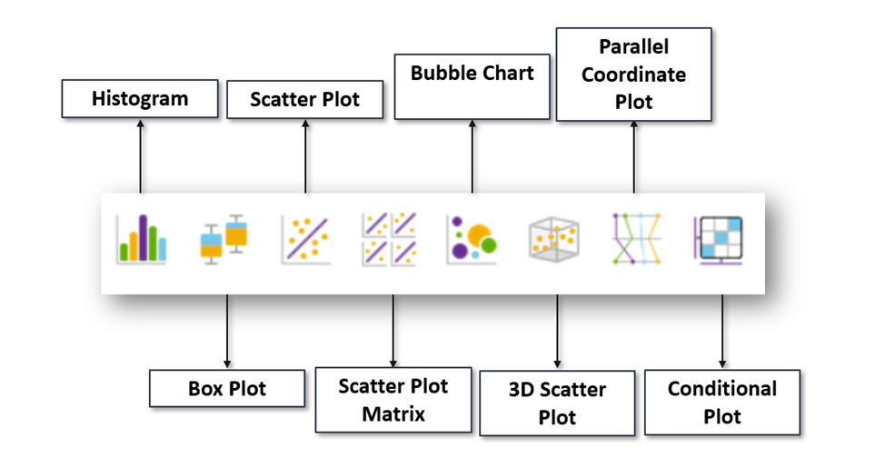
Figure 2.4: Types of graphics in GeoDa
3.3.1 Histogram
Histogram shows the meanings of one variable for each chosen object. You have to push the histogram button on the control panel and to choose the variable you need. If you want to create histogram not for all objects, but for concrete ones, you have to choose them either from the table or from the map. In that case the histogram will show the meanings of the variable for all objects and for chosen ones. To open the table, you have to push the button on the control panel. To chose other colors for the histogram or to export it as an image, you have to click it with the right button and to choose the option you need. This works for all types of graphics in GeoDa.
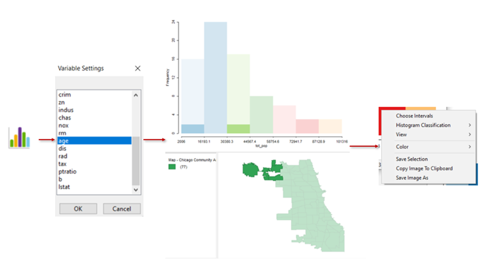
Figure 2.5: Creating Histogram in GeoDa
3.3.2 Box plot
Boxplots are created to represent the distribution of a numeric variable. The graphic reflects maximum and minimum values, median, first and last quantiles and p-values at the same time. To create boxplot, you also just have to push the button on the control panel and to choose the variable you need. Boxplot also has some numeric characteristics for easier interpretation.
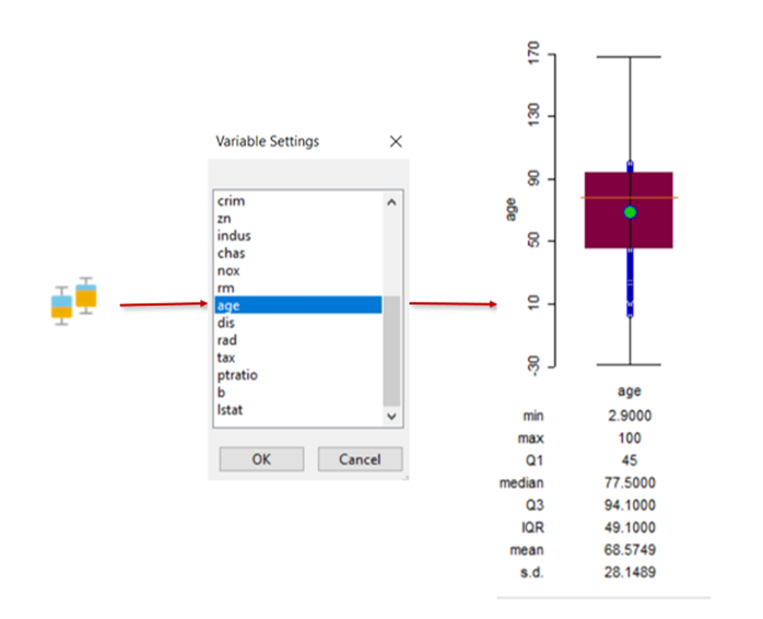
Figure 2.6: Creating Box plot in GeoDa
3.3.3 Scatter plot
Scatter plot is based on using Cartesian coordinates to display values for typically 2 variables for a dataset. There’re 3 types of Scatter plots in GeoDa. To create each of them, you still have to push a specified button on a control panel and create the variables. For classical scatter plot you’ll have to choose 2 of them. The 3D Scatter plot uses the 3-dimensial representation for 3 variables. Finally, the Scatter plot Matrix is a grid of scatter plots used to visualize bivariate relationships between combinations of variables. Here you can choose more than 2 or 3 variables for comparison, if you need. To create scatter plots, you also just have to push the button on the control panel and to choose the variable you need.
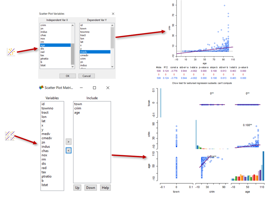
Figure 3.1: Creating Scatterplot and Scatterplot Matrix in GeoDa
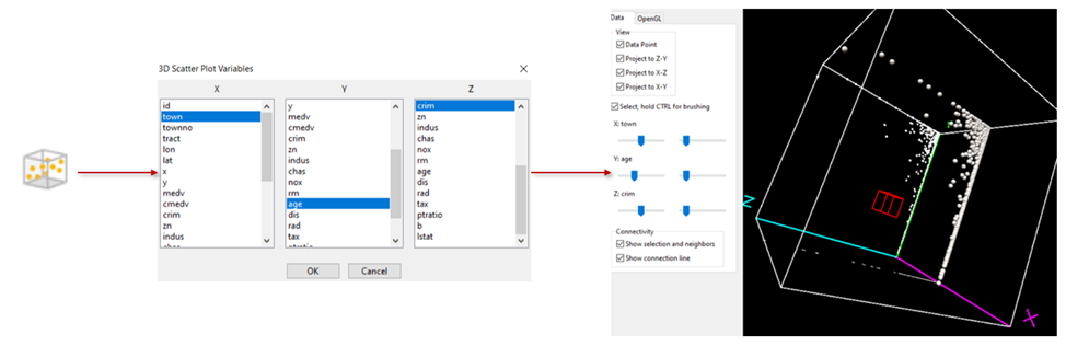
Figure 3.2: Creating 3D Scatterplot in GeoDa
3.3.4 Bubble Chart
A bubble chart is a type of data visualization that uses circles (bubbles) to represent data points in a two-dimensional plot. It is similar to a scatter plot, but uses bubbles instead of dots. Typically, a bubble chart shows the values of three numeric variables, with each circle representing an observation and its position on the plot indicating the values of two other variables. To create bubble chart, you also have to push the button on the control panel and to choose the variable you need.
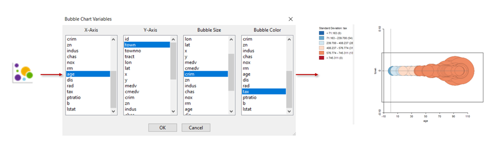
Figure 3.3: Creating Bubble Chart in GeoDa
3.3.5 Parallel coordinates plot
Parallel coordinates plot is a common way of visualizing and analyzing high-dimensional datasets. A point in n-dimensional space is represented as a polyline with vertices on the parallel axes and the position of the vertex corresponds to the coordinate of the point. To create it, you have to push the button on the control panel and to choose the variable you need.
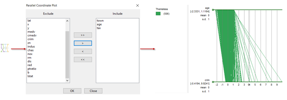
Figure 3.4: Creating Parallel coordinates plot in GeoDa
3.3.6 Conditional plot
- Conditional plot consists of two variables conditional on the value of a third variable. You can create a map, a histogram, a scatter plot or a boxplot, using the button on a control panel. You’ll have to choose 3 variables and get 9 graphics, showing their dependencies.
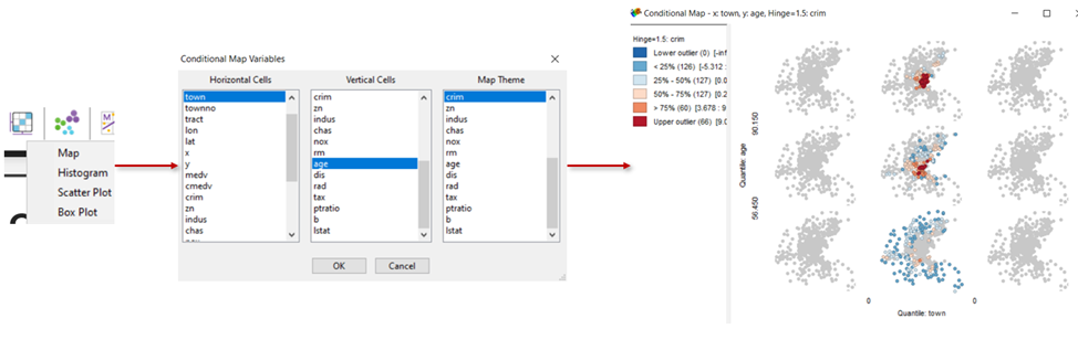
Figure 3.5: Creating a Conditional plot in GeoDa
3.4 Practical exercise
To check yourself after this lesson you have to built 3 Graphics for the observations with the towno=27. 1. You have to create a histogram to analyze distances to Boston employment centers (dis); 2. You have to create a histogram to analyze per capita crime (crim) and fix in *.txt file the minimum, maximum, mean and median values of the variable; 3. You have to create a bubble chart to analyze the dependencies between such variables as age (x-axes), dis (y-axes), crim (bubble-size) and indus (bubble-color). The result of your task must be represented by a txt-file with statistical parameters and 3 png-files with graphics.