7 Spatial statistics in GeoDa. Part 2

Lesson summary

7.1 Previous lection

In the previous lesson you have learned why spatial dependence is important, also you have learned some basics including Moran’s Index. There are two types of Moran’s statistics. First is global Moran’s test. This test allows us to assess the statistical relationship between the value of the indicator in each location and in neighboring locations. Second is local Moran’s test. Using this method you can create maps which can illustrate the spatial statistical differences between variables. In general, Moran’s Index is needed when you need to prove the importance of connection between two variables. But also there are a lot of different methods to explore the data.

7.2 Theme of the lesson

In this lesson you will study the additional spatial statistics methods represented in GeoDa:

• Joint Count
• Local Geary
• Quantile LISA
• Spatial Correlogram
• Linear regression

7.3 Contiguity and spatial weights

Contiguity and spatial weights are the two things which you can use in the weight manager in the next cases.

In its simplest form, the spatial weights matrix expresses the existence of a neighbor relation as a binary relationship, with weights 1 and 0. Usually this matrix is very sparse with a lot of zeros in it.

Contiguity means that two spatial units share a common border of non-zero length. Operationally, we can further distinguish between a rook and a queen criterion of contiguity, in analogy to the moves allowed for the such-named pieces on a chess board.

7.4 Joint count methods

7.4.1 Theoretical basis

Joint Count method is a technique for processing discrete variables, especially for binary variables. It is used to identify clusters in binary variables by means of the local joint count statistics. The statistics consists of counting the joins that correspond to occurrences of value pair at neighboring locations. Mathematic representation of this method: \[ BB_i = x_i\sum_{j}{w_i w_j}x_j \] This equation means that Joint Count is a sum of neighbors of \(x_i\) which are have the same value that x. In conclusion, you can use these methods to determine if there is a spatial connection between events or they are distributed in the random way. ### Implementation in GeoDa To create map using this method you have to create a weight matrix first: 1. Open the Weights Manager 2. Choose “Create” 3. Select an ID variable in your dataset 4. Choose type of contiguity 5. Choose variable as spatial weight 6. Save the weight data In the end you will see similar picture:

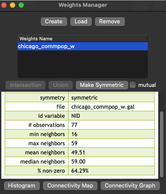
Figure 2.1: Weights Manager

After creating the weight matrix you can make the map. The only available option is a significant map. 1. Open Local Joint Count in Space bar menu 2. Select the variable you want to explore

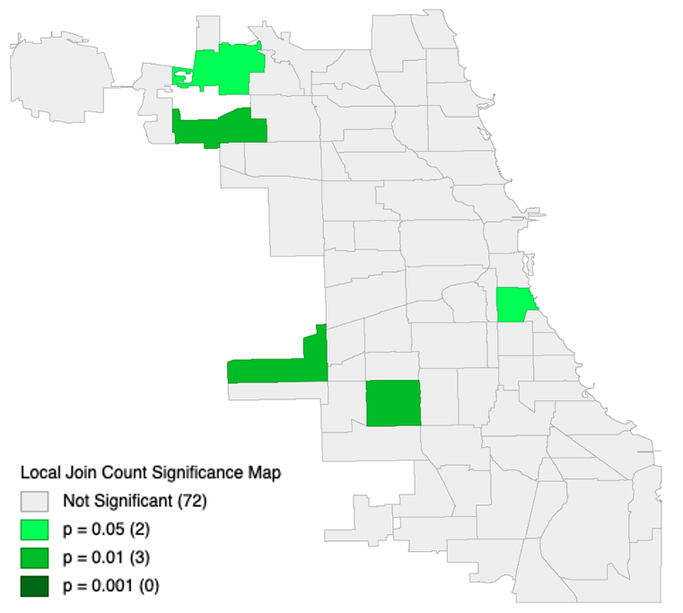
Figure 2.2: Local Join Count Significance Map

This map represents a spatial significance of negative population growth in Chicago city, IL. It means that the regions colored in green have strong connection between their location and decreasing its population. The reason can be different, but this reason stronngly affects to them.

7.5 Local Geary

7.5.1 Theoretical basis

Local Geary is a method to find the spatial autocorrelation through dissimilarity of data. It means that small values of the statistics suggest positive spatial autocorrelation, whereas large values suggest negative spatial autocorrelation. It can be more precise that Local Moran test in some cases because of differences in attribute similarity.

7.5.2 Implementation in GeoDa

First, you need to prepare the weight matrix like in the previous step. Next step is to open “Local Geary” in Space bar menu and select the variable. In spite of Joint Count method you can choose two options for the maps. First is a cluster map which is a representation of attribute dependencies. Second variant is a significance map like in the Joint Count method.

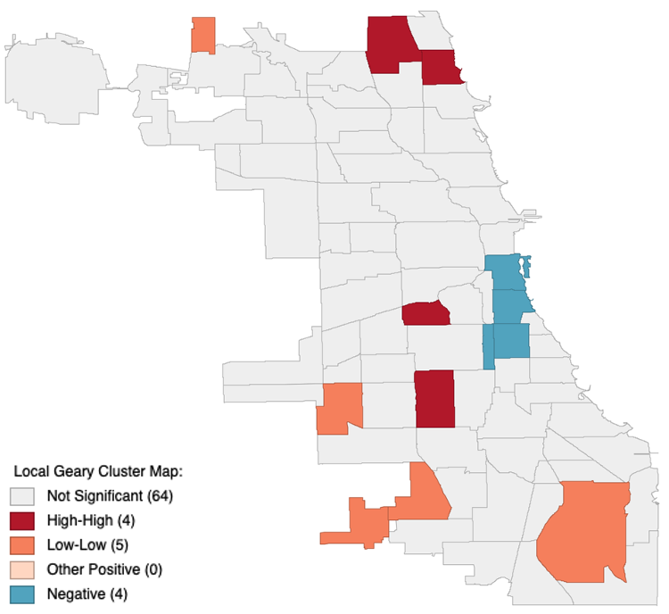
Figure 2.3: Local Geary Cluster Map. Tuberculosis in Chicago

The cluster map is a great way to show spatial dependencies connected with attributes. Theoretically there are five categories. First category is a “Not Significant”. It means that there is no dependency between attribute and spatial component. Second category is a “High-High”. It this category there is a strong positive connection between attribute and location. The next category is a “Low-Low”. This category represents straight, but negative connection. It means that surrounding area has the similar low values of the attribute like this regions. The fourth category represents low significant straight connection. The last category is about negative connection between this region and surrounding area. But what it means in the practical way? Map shown in the top represents the connection between location and tuberculosis spreading, but let’s imagine that it is a cost of the flat in condominium. In the areas with “High-High” category there are high prices both in the colored regions and surrounding area. In the “Low-Low” areas cost is low in the similar way. Despite of this places the areas with negative connection have a potential for a good deal. You need to estimate is this place has a lower price that in surrounding area or not. If it is you can save your money.

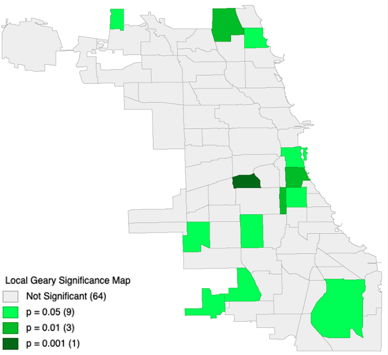
Figure 2.4: Local Geary Significance Map. Tuberculosis in Chicago

The Significance map represents power of the connection between attributes and spatial location like in the Joint Count method.

7.6 Quantile LISA

7.6.1 Theoretical basis

Quantile LISA or quantile local spatial autocorrelation is a method to find spatial autocorrelation between two or multiple continuous variables. Linear association measured by Bivariate Local Moran suffers from the location problem. Quantile LISA added a spatial component for measuring correlations. More often it is used when the focus is on extremes of the distribution.

7.6.2 Implementation in GeoDa

First do the steps like in Joint Count and Local Geary methods with creation of spatial weights. Next you need to select the variables and quantiles for analysis.

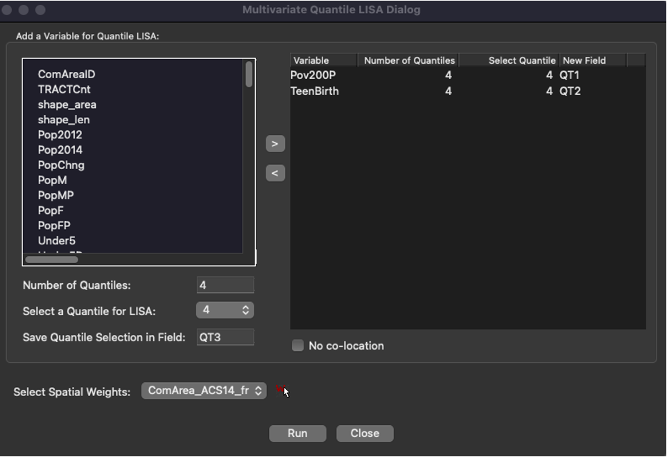
Figure 2.5: Selecting quantiles and number of quantiles

Let’s explore how extreme poverty is connected with teen pregnancy. Select the category and use the last quantile. In this case we will see the dependency between proportion of people with income less than 50% of povery minimum and number of teen pregnancies.

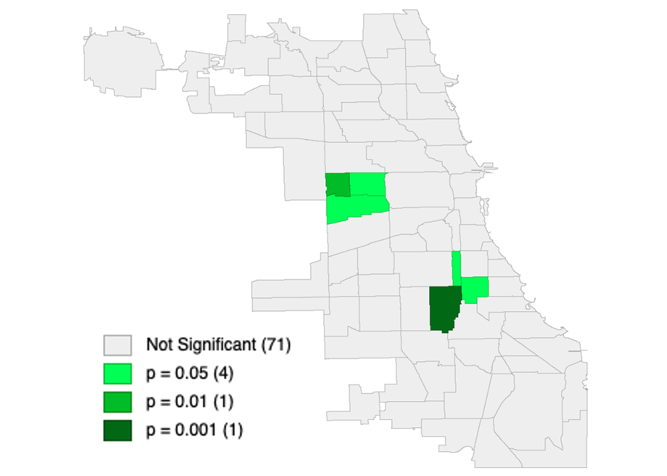
Figure 2.6: Quantile LISA Significance Map. Connection between extreme povery and number of teenage pregnancies

Like in the previous methods we can make a significance map representing power of spatial correlation between attributes.

7.7 Spatial correlogram

7.7.1 Theoretical basis

A non-parametric spatial correlogram is an alternative measure of global spatial autocorrelation that does not rely on the specification of a spatial weights matrix. Instead, a local regression is fit to the covariances, or correlations computed for all pairs of observations as a function of the distance between them. The non-parametric correlogram is computed by means of a local regression on the pairwise correlations that fall within each distance bin. The number of bins determines the distance range of each bin. This range is the maximum distance divided by the number of bins. The more bins are chosen, the more fine-grained the correlogram will be

7.7.2 Implementation in GeoDa

First choose Spatial correlogram in space bar tools. Next choose the data. You will see the “Correlogram Parameters” menu.

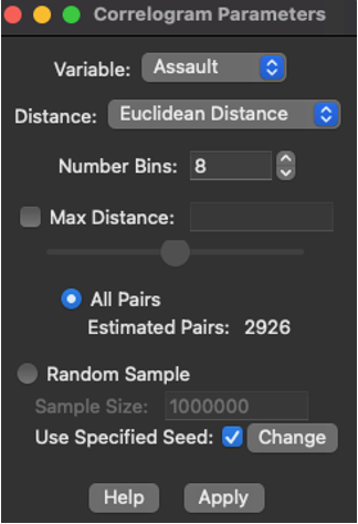
Figure 3.1: Selecting quantiles and number of quantiles

You should choose variable for analysis and number of beans first. Note that there is an option that it will be no spatial dependency between distance of the regions and attribute values.

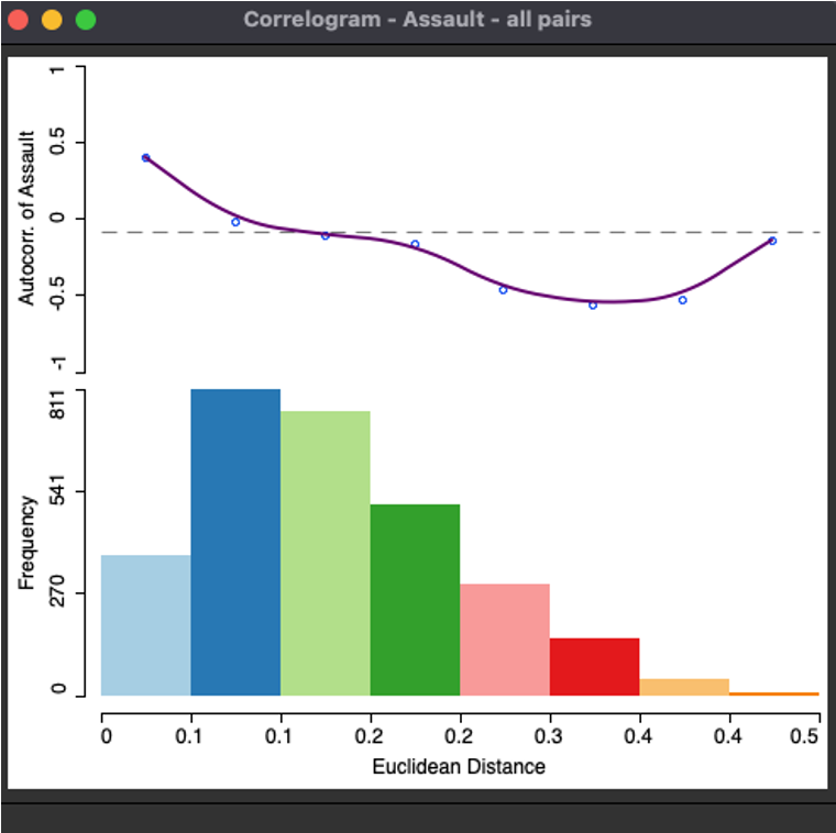
Figure 3.2: Correlogram between number of assaults and distance

As you can see there is a little dependency between this two variables. It means that number of assaults decreases with increasing distance parameter between two regions. It can representate the fact that unfortunate districts are close to each other and they are located in the big distance from prosperous ones.

7.8 Regression

7.8.1 Theoretical basis

Regression analysis is a set of statistical processes for estimating the relationship between a dependent variable and one or more independent variables. In the standard regression parameters of the model are constant. It means that there is no difference in spatial dependence between variables. To solve this problem, you can use geographically weighted regression. In this method weights are defined for every location individually. In the mathematical point of view weight coefficient matrix is used where close points have higher influence rate than far ones.

7.8.2 Implementation in GeoDa

• Note that regression is in different menu than other spatial statistics tools
• You need to select dependent and independent variables
• You may add additional weights file

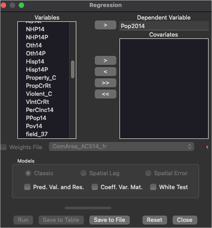
Figure 3.3: Settings of the regression

After processing you will see the Regression Report.

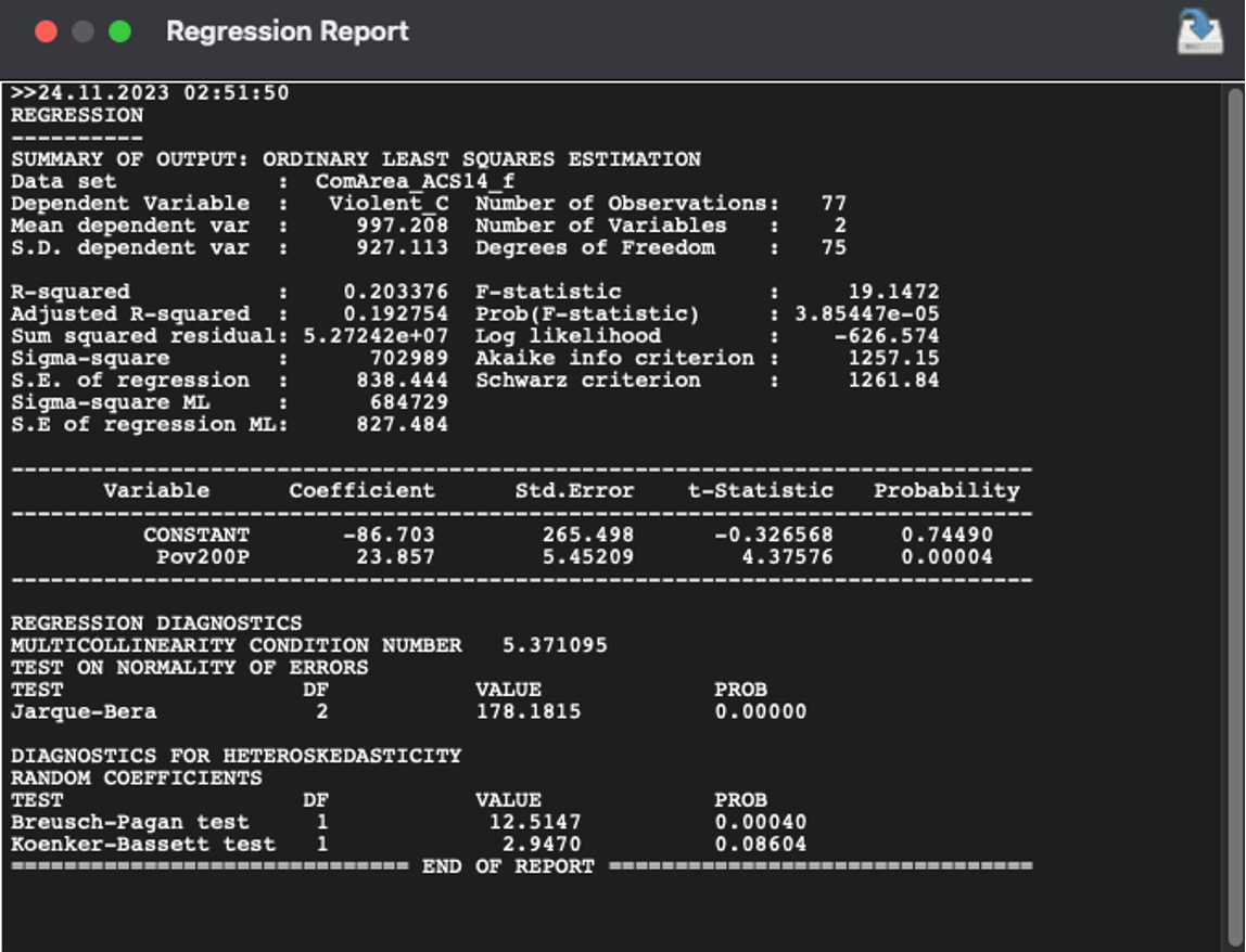
Figure 3.4: Regression Report

There are two key points in it. First: R-squared – statistical measure that determines the proportion of variance in the dependent variable that can be explained by the independent variable. Second: F-value – statistical measure where the null hypothesis is that all the regression coefficients are equal to zero. In this case regression can’t predict the model of connection between data.

7.9 Conclusion

• Use Joint Count methods if you need to process with binary data
• Use Local Geary methods if you need to describe the contiguous data and find similarity and dissimilarity areas
• Use Quantile LISA if you need to process contiguous data with multiple variable and find an autocorrelation
• Use spatial correlogram if you need to find correlation between differences of variable and different distances
• Use a regression to prove your concept

7.10 Task

• Explore the spatial correlation between poverty with cancer deaths per 100 000 people in Chicago region.
• Use this dataset: https://geodacenter.github.io/data-and-lab/comarea_vars/
• Use Pov200P as an independent variable and CancerAll as dependent variable
• Try Local Geary and Quantile LISA to find autocorrelation and make map. In the end use regression tool to make a conclusion between their dependency
• Describe the result which you get with significance maps and regression report